Getting Started

A first example

The following example covers the basic workflow of the package. A GP prior is placed on a set of basis points and wrapped in a Kalman filter. The filter learns an unknown scalar function from noisy samples, one sample at a time, and the learned function is then evaluated at arbitrary inputs together with its uncertainty.

using RecursiveGPs     # RGP, ExtendedKalmanFilter, predict_gp
using AbstractGPs      # kernels
using StaticArrays     # static vectors and matrices for the filter
using LinearAlgebra    # diag
using Random
using CairoMakie

1. Data

100 samples of $f(u) = 0.5u + 0.1\sin(2\pi u)$ on $[0.1, 0.8]$, with sensor noise of standard deviation 0.005:

Random.seed!(42)
f(u) = 0.5u + 0.1 * sinpi(2u)
σn = 0.005

us = 0.1 .+ 0.7 .* rand(100)
ys = [SA[f(u) + σn * randn()] for u in us]

2. GP prior

An RGP is defined by a kernel and a set of basis points that covers the input range. Here the kernel is a squared exponential with variance 0.1 and length scale 0.4, close to the maximum-likelihood values found in the Hyperparameter Tuning tutorial. The basis has 21 points on $[0, 1]$:

kernel = 0.1 * with_lengthscale(SEKernel(), 0.4)
b0 = collect(range(0, 1, length = 21))

rgp = RGP(kernel, b0)

A mean function can be passed as the first argument, for example RGP(u -> 0.5u, kernel, b0).

3. Filter

The filter state is the vector of GP values at the basis points, initialised with the prior mean and covariance. The function is constant in time, so the dynamics are the identity. The measurement is the GP mean at the input, and the measurement noise is the residual variance of the GP plus the sensor noise variance σn^2:

kf = ExtendedKalmanFilter(rgp; σn)

Models with several GPs or with physical states use the multi-component constructor, which takes the dynamics and measurement functions explicitly. The tutorials show how.

4. Learning

Each call kf(u, y) runs one prediction and one correction step:

for (u, y) in zip(us, ys)
    kf(u, y)
end

5. Prediction

predict_gp returns the posterior mean and covariance of the function at any query points:

b = collect(range(0, 1, length = 200))
post = predict_gp(kf, b)

μ = post.μ               # posterior mean
σ = sqrt.(diag(post.Σ))  # posterior standard deviation

predict_kf returns the predicted measurement at a single input, including the measurement noise.

fig = Figure(size = (800, 450))
ax = CairoMakie.Axis(fig[1, 1]; xlabel = "u", ylabel = "f(u)")

band!(ax, b, μ .- 2σ, μ .+ 2σ; color = (:orange, 0.3), label = "Posterior μ ± 2σ")
lines!(ax, b, f.(b); label = "Ground truth")
lines!(ax, b, μ; color = :orange, label = "Posterior μ ± 2σ")
scatter!(ax, us, first.(ys); color = :red, markersize = 6, label = "Training data")

xlims!(ax, extrema(b))
ylims!(ax, 0.0, 0.55)
axislegend(ax; position = :rb, merge = true)
fig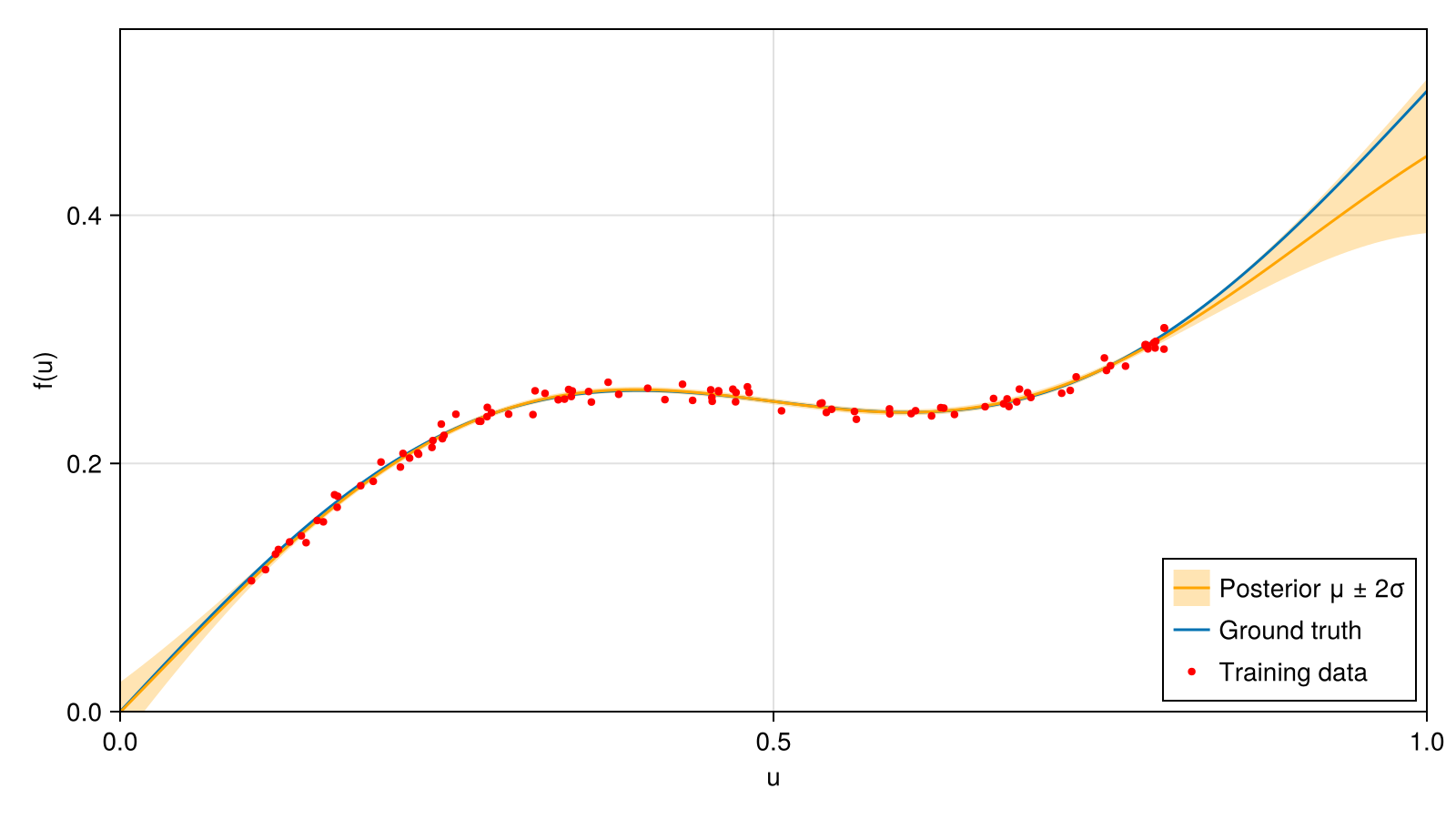

Within the training range, $0.1 \le u \le 0.8$, the posterior mean follows the ground truth and the band contains it. Outside this range the band widens, and the estimate relies increasingly on the prior.

Next steps

• Tutorials: several GPs in one model, hyperparameter tuning, and an RGP inside a physical model.
• Mathematical Background: derivation of the recursive GP.
• API Reference: all exported functions.