Multi-Component RGPs

A measurement can depend on several unknown functions. Each function is represented by its own RGP, and one extended Kalman filter learns all of them from the same measurements.

Problem Setup

We observe

\[y_t = f_1(u_1) + u_2 \cdot f_2(u_1)\]

where $f_1(b) = e^b$ and $f_2(b) = 0.1 + 0.5b + 0.1\sin(2\pi b)$. The input $u_2$ is a scalar gain. Neither function is observed directly, only their weighted sum. The two functions can be separated because $u_2$ varies between measurements. The measurements contain sensor noise with standard deviation 0.01.

using RecursiveGPs
using AbstractGPs
using StaticArrays
using ComponentArrays
using LinearAlgebra
using Random
using CairoMakie

Dataset

Random.seed!(123)

f1(b) = exp(b)
f2(b) = 0.1 + 0.5 * b + 0.1 * sinpi(b * 2)

n   = 100
ts  = collect(range(0, 100, n))
u1  = 0.1 .+ rand(n) / 1.5
u2  = 0.2 .* randn(n)
gt  = @. f1(u1) + u2 * f2(u1)
σn  = 0.01

ys  = [SA[y + σn * randn()] for y in gt]
us  = [(; u1 = u1[i], u2 = u2[i]) for i in 1:n];

Define RGP Components

Each latent function gets its own RGP with a separate kernel. Both share the same basis-point grid.

b0 = collect(0:0.05:1)

rgp_a = RGP(0.8 * with_lengthscale(SEKernel(), 0.3), b0)   # models f1
rgp_b = RGP(0.1 * with_lengthscale(SEKernel(), 0.3), b0)   # models f2

components = (; a = rgp_a, b = rgp_b);

Dynamics, Measurement, and Noise

The KF state is the concatenation of the two component states: $x = [g^{(a)}; g^{(b)}]$.

Dynamics: identity, since both functions are constant in time.

dynamics(x, u, p, t) = x

dynamics (generic function with 1 method)

Measurement: combine component outputs according to the observation model. xid axes are stored in p for slicing x into named components.

function measurement(x, u, p, t)
    (; xid) = p
    xc = ComponentVector(x, xid)
    μ1 = measurement_gp(p.a, xc.a, u[1])
    μ2 = measurement_gp(p.b, xc.b, u[1])
    return (μ1 + u[2] * μ2) |> SVector{1}
end

measurement (generic function with 1 method)

Noise covariance: the residual variances of both GPs, weighted by the squared coefficients of the measurement, plus the sensor noise variance.

function R2(x, u, p, t)
    r1 = uncertainty_gp(p.a, u[1])
    r2 = uncertainty_gp(p.b, u[1])
    return (r1 + u[2]^2 * r2 + σn^2) |> SMatrix{1, 1}
end

R2 (generic function with 1 method)

Construct and Train the Filter

kf = ExtendedKalmanFilter(components, dynamics, measurement, R2)

for (u, y) in zip(us, ys)
    kf(u, y)
end

Predict Output

pred_μ = Float64[]
pred_σ = Float64[]

for u in us
    p = predict_kf(kf, u)
    push!(pred_μ, p.μ[1])
    push!(pred_σ, sqrt(p.Σ[1, 1]))
end

Plot Output vs Ground Truth

fig1 = Figure(size = (800, 450))
ax1  = CairoMakie.Axis(fig1[1, 1]; title = "Combined RGP output", xlabel = "t", ylabel = "y")

lines!(ax1,  ts, gt;     label = "Ground truth")
lines!(ax1,  ts, pred_μ; color = :orange, label = "Posterior μ ± 2σ")
band!(ax1,   ts,
      pred_μ .+ 2 .* pred_σ,
      pred_μ .- 2 .* pred_σ;
      color = (:orange, 0.3), label = "Posterior μ ± 2σ")
scatter!(ax1, ts, first.(ys); color = :red, markersize = 4, label = "Training data")

xlims!(ax1, extrema(ts))
Legend(fig1[2, 1], ax1; orientation = :horizontal, framevisible = false, merge = true)
fig1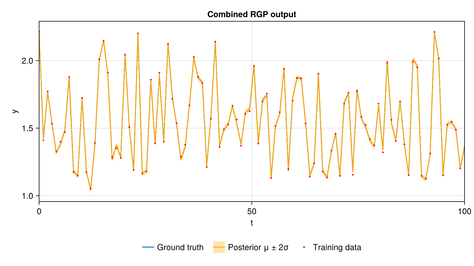

Extract Individual Component Predictions

Use predict_gp with a component symbol to query each latent function independently.

b_plot = collect(range(0.0, 1.0, length = 100))

pred_a = predict_gp(kf, b_plot, :a)
pred_b = predict_gp(kf, b_plot, :b)
σ_a    = sqrt.(diag(pred_a.Σ))
σ_b    = sqrt.(diag(pred_b.Σ))

fig2 = Figure(size = (800, 420))
axs  = [CairoMakie.Axis(fig2[1, i]; xlabel = "b") for i in 1:2]

axs[1].title = "Component a:  f₁(b) = exp(b)"
axs[1].ylabel = "f₁(b)"
lines!(axs[1], b_plot, f1.(b_plot);   label = "Ground truth")
lines!(axs[1], b_plot, pred_a.μ;      color = :orange, label = "Posterior μ ± 2σ")
band!(axs[1],  b_plot,
      pred_a.μ .+ 2 .* σ_a,
      pred_a.μ .- 2 .* σ_a;
      color = (:orange, 0.3), label = "Posterior μ ± 2σ")
scatter!(axs[1], u1, f1.(u1); color = :red, label = "Training inputs")

axs[2].title = "Component b:  f₂(b) = 0.1 + 0.5b + 0.1sin(2πb)"
axs[2].ylabel = "f₂(b)"
lines!(axs[2], b_plot, f2.(b_plot);   label = "Ground truth")
lines!(axs[2], b_plot, pred_b.μ;      color = :orange, label = "Posterior μ ± 2σ")
band!(axs[2],  b_plot,
      pred_b.μ .+ 2 .* σ_b,
      pred_b.μ .- 2 .* σ_b;
      color = (:orange, 0.3), label = "Posterior μ ± 2σ")
scatter!(axs[2], u1, f2.(u1); color = :red, label = "Training inputs")

xlims!.(axs, Ref(extrema(b_plot)))
Legend(fig2[2, 1:2], axs[1]; orientation = :horizontal, framevisible = false, merge = true)
fig2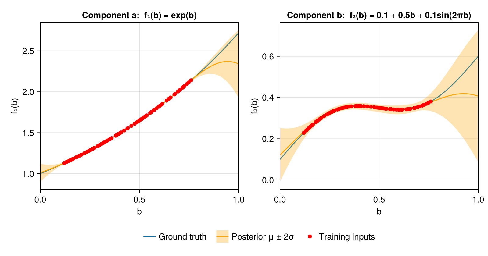

Both posteriors contain the ground truth within the training range. The band of $f_2$ is wider than that of $f_1$, because $f_2$ enters each measurement only through the small gain $u_2$.

This page was generated using Literate.jl.